Real systems in nature, including computer systems, economy, physics, etc. may reach a point where the changes of the cost outweigh the performance changes with respect to some tunable parameter. This renders the further changes “not worth it” and sometimes maybe even harmful. Therefore, in many cases it is important to manage tradeoffs between the cost and performance. One particular point of interest in reaching a balanced tradeoff is called the knee or the elbow. Various definitions of a knee exist but the most popular one defines the knee as a point in which a graph obtains maximum curvature, or equivalently, an osculating circle at that point has the smallest radius.
Knee searching is quite important operation. In this post I’ll describe the method I personally developed: the C-method.
Description
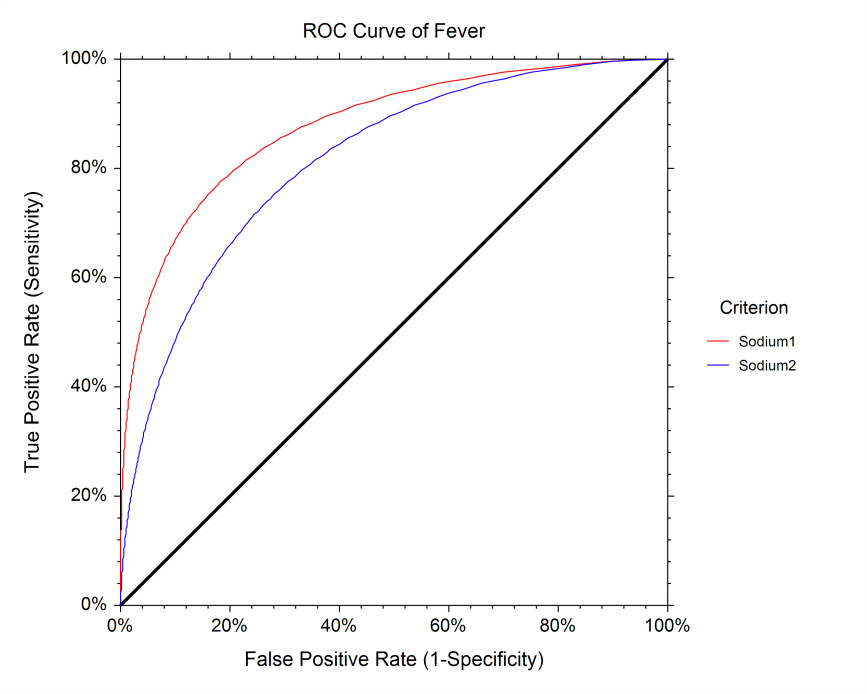
Figure 1: A typical trade-off curves. A balancing point, a.k.a. a knee, might be found at 30% for the blue curve and below 20% for the red curve.
It all started with an observation: many tradeoff curves I’ve come across with vaguely look like x1 or 1−x1. The most generic form of this equation is therefore:
f(x)=a+x+cb
It has three shape parameters: a, b, and c, and fitting these parameters should be enough. However, I felt that this is way too much degrees of freedom; if I restrict the function with some constraints, I should ideally get the functional form with only one shape parameter. Most of my experience was that most of the time the function graphs are anchored to pass through the points (0,0) and (1,1), so I restricted the function such that f(0)=0 and f(1)=1.
Constraint 1
When f(0)=0 is fed into the equation form results in a relation:
0=f(0)b=a+0+cb==a+cb=−ac
Feeding the relation back into the equation results with:
When c<0, the curve “flips”, meaning the curve avoids the unit square.
I decided I did not like this as, while perfectly mathematically correct, it does not match my intuition at all to me, ideally limc→0 should go to x and limc→+∞ should go to x. Also, I would like to restrict c to all positive reals.
All of my problems are solved with a following substitution: c→ec1.2 Doing the substitution gave me:
Much better, IMHO. It’s got a nice visual which is easy to remember. The only difference is the parantheses The GeoGebra plugin animating the function as the c parameter changes
Analysis
limc→−∞=x, which was what I wanted
limc→+∞=1, which was also what I wanted
Flipping is now disabled
How to use it to find a knee?
Three ways: the intuitive way, the technical way, and the hacky way.
The intuitive way
The intuitive way starts with an observation that the function graph is symmetric with respect to the line y=1−x. Intersecting the graph with the line gives:
The quadratic equation has two solutions, however I must disregard one of them as it’s smaller than 0. Therefore, the knee point is at:
x=ec−1+1+ec
The technical way
The second way is way more technical as it involves a lot of calculus. If I define a curvature function K(x)=(1+f′2)23f′′, I could find an extreme point by setting dxdK(x)=0. Before substitution, let’s play with the expression first:
which is what we’ve already obtained in the last step, which is great!
The hacky way
The third approach is rather hacky. By invoking a Mean Value Theorem, we know there must be a point on the curve of f(x) in which the slope of the tangent is equal to the slope of the secant between (0,0) and (1,1). That slope is, obviously, 1. Therefore, finding the derivative and evaluating it with 1 gives:
dxdf(x)dxdxec+1x(ec+1)(xec+1)2ec+1=1=1=1
which, once again, results with x=ecec+1−1.
After three different proofs, I guess it’s safe to say that x=ecec+1−1 is a good estimator of the theoretical knee.
Estimating the c
After this theoretical derivation, the next problem is fitting the c coefficient to the real world data, N-dimensional vectors x and y. The first, and only insofar, fitting procedure I’ve come up with is the ordinary least squares: minimization of:
These equations are then simply converted to an update rule:
cn+1←cn−∂c2∂2E∂c∂E
which works for any starting value c0. This procedure is repeated until a satisfactory level of precision is reached. The resulting shape parameter c is then fed into the equation above to get the knee point. Optionally, one can also calculate which of the input xi’s is the closest to the theoretical knee and denote that particular xi as a knee.
What’s next?
I would be most happy if I found that f′(x) could be written in terms of f(x) or f′′(x) could be written in terms of f′(x) in a nice manner (just like the derivative of a sigmoid). However, I am not that good in algebra.
Efficient implementation. Currenctly it’s implemented as a brain-dead verbatim implementation using only numpy. I’m even calling other functions to calculate the derivatives, which turned out to be rather slow. If I ever accomplished the point above, this would easily follow.
Sometimes, the graphs which are in need of the knee/elbow search do not behave like 1−x1 but more like 1−x21 or 1−x1. It would be great to investigate such possibilities and allow for one more shape parameter.
Thank you for your time and until next time,
Marijan Smetko
QED
However it should be emphasised that this was only possible because the degree of the denominator was 1. Future generalizations which would allow for a different exponent ↩
 to me, ideally should go to and should go to . Also, I would like to restrict to all positive reals.