Average entropy of a discrete probability distribution (part 1)

In this blogpost I will present my own little research in maths: the search for an expression of the expected value of an n-dimensional discrete probability distribution.

Average entropy

The story begins while I was learning Information Theory at my uni. We talked about the entropy of a binary random variable. A binary random variable is a variable which only ever has two outcomes, 0 or 1.¹. The pmf of a Bernoulli variable is

$$\begin{pmatrix} 0 & 1 \\ 1-p & p \end{pmatrix}$$

The entropy of a Bernoulli variable is then²

$$E\left[X\right] = -p\ln\left(p\right) - \left(1-p\right)\ln\left(1-p\right)$$

Now for the question: what is the average entropy of a Bernoulli variable? If we were to pick a lot of random $p$, calculated the entropy and averaged all of them, what number would we get as a result? We could just integrate over all $p$’s, and divide by the size of the space of $p$. To borrow some physics intuition, to calculate the average density of an object, you first calculate the mass of an object by integration, and then divide by the size of the object (i.e. its volume). Here the “size” of the space happens to be $1$. Anyways:

$$\begin{align*} \overline{E_2} &= \frac1{1-0}\int_{0}^{1}{E(p)\mathrm{d}p} =\\ &= -\int_{0}^{1}{p\ln\left(p\right) + \left(1-p\right)\ln\left(1-p\right) \mathrm{d}p} =\\ &= ... \mathrm{use\ photomath\ or\ sth} ...\\ &= \frac12 \end{align*}$$

Two’s a company, three’s a crowd

Let’s move a step up. What if we picked a random 3-dimensional “Bernoulli” and calculated it’s entropy. What is the average (or expected) entropy of a random 3-dimensional variable?

First, let’s define some stuff. 3-d Bernoulli variable does not exists, as the term Bernoulli is reserved for 2-dimensional case excusively. Higher dimensional random variables are caled Multinoulli, presumably because someone was feeling particularly creative that day. It’s entropy is calculated with:

$$E[X] = -\sum_{i=1}^{N}{p_i\ln(p_i)}$$

$$E_3(p, q) = -p\ln(p) - q\ln(q) - (1-p-q)\ln(1-p-q)$$

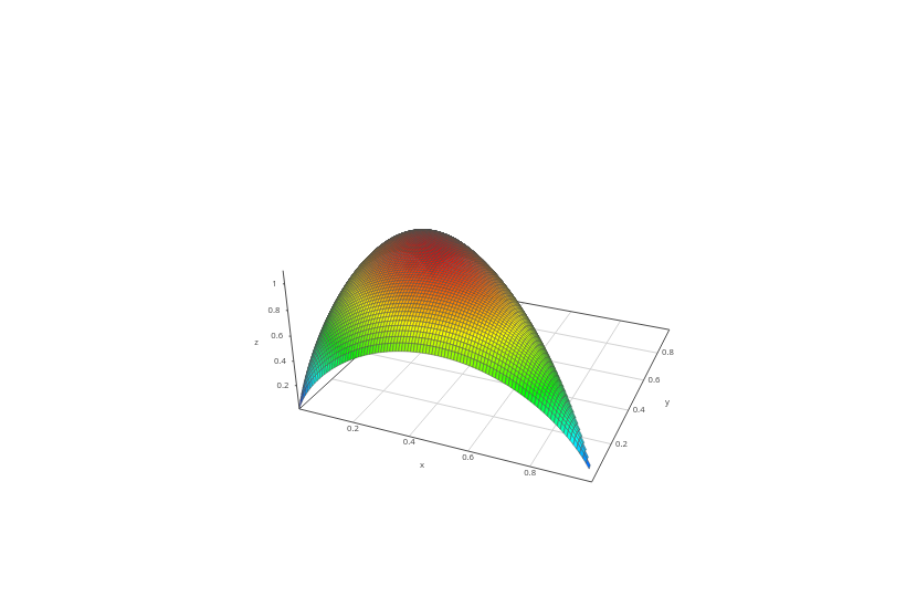
How do we calculate the average entropy of this? Using the same process as above: integrate the function and divide by the “size” of the function’s domain. Here, the domain is a 2D triangle⁴ determined by the lines $p \ge 0$, $q \ge 0$, $p+q \le 1$. This triangle is exactly one half of the unit square, so it has to have an area of $\frac12$. The average entropy of a 3-dimensional multinoulli variable is:

$$\begin{align*} \overline{E_3} &= \frac1{\frac12}\int_{0}^{1}{\int_0^{1-p}{E(p, q)}{\mathrm{d}q}}{\mathrm{d}p} =\\ &= \frac1{\frac12}\int_{0}^{1}{\int_0^{1-p}{-p\ln(p) - q\ln(q) - (1-p-q)\ln(1-p-q)}{\mathrm{d}q}}{\mathrm{d}p} =\\ &= ... \mathrm{use\ wolfram\ alpha\ or\ sth} ...\\ &= \frac5{12} \end{align*}$$

Okay, no visible pattern so far. To quote data scientists, “More data is needed!”. To dimension no.4

Three is a crowd, four is unthinkable. Literally

Let’s try to find out what happens if we calculate the average entropy of a random 4-dimensional multinoulli variable. This is something we usually cannot even imagine, however it’s quite feasible due to maths. The recipe is the same: integrate and divide by the volume of the domain.

First, we’ll have to add one more variable to the calculation of entropy:

$$E_4(p, q, w) = -p\ln(p) - q\ln(q) - w\ln(w) - (1-p-q-w)\ln(1-p-q-w)$$

• $p \ge 0$
• $q \ge 0$
• $w \ge 0$
• $p+q+w \le 1$

and its volume is $\frac16$. (This is a good exercise for the reader btw)

And now for the integral…

$$\begin{align*} \overline{E_3} &= \frac1{\frac16}\int_{0}^{1}{\int_0^{1-p}{\int_0^{1-p-q}{E(p, q)}{\mathrm{d}w}}{\mathrm{d}q}}{\mathrm{d}p} =\\ &= \frac1{\frac16}\int_{0}^{1}{\int_0^{1-p}{\int_0^{1-p-q}{-p\ln(p) - q\ln(q) - w\ln(w) - (1-p-q-w)\ln(1-p-q-w)}{\mathrm{d}w}}{\mathrm{d}q}}{\mathrm{d}p} =\\ &= ... \mathrm{? ? ? ? ?} \end{align*}$$

>>> from sympy import symbols, integrate, ln, simplify
>>> p, q, w = symbols('p q w', real=True)
>>> E = -p*ln(p)-q*ln(q)-w*ln(w)-(1-p-q-w)*ln(1-p-q-w)
>>> domain_volume = 1/6
>>> res = integrate(f, (w,0,1-p-q), (q,0,1-p), (p,0,1))
>>> # seven hungry years later
>>> print(result.real / domain_volume)
13/12

The result is $\frac{13}{12}$.⁵ No obvious pattern yet.

And also, these integral solving functions take progressively more and more time. Running it for 2-dimensional case took ~4sec, for 3-dimensional case took ~20 sec, and for 4-dimensional case it took a whooping 163 sec to get an anwser. If we assume it’s a factorial growth, we’re looking forward to ~10 minutes for 5-dimensional case and ~2h for 6 dimensions.

I could, in theory, buy a better laptop but it won’t help me much. Therefore, we’ll need to look for other methods that trade computation speed for absolute precision. See you in the next part.